Transformée de Fourier

Passage Série de Fourier –> Transformée de Fourier

Augmentons la période T de notre signal périodique :
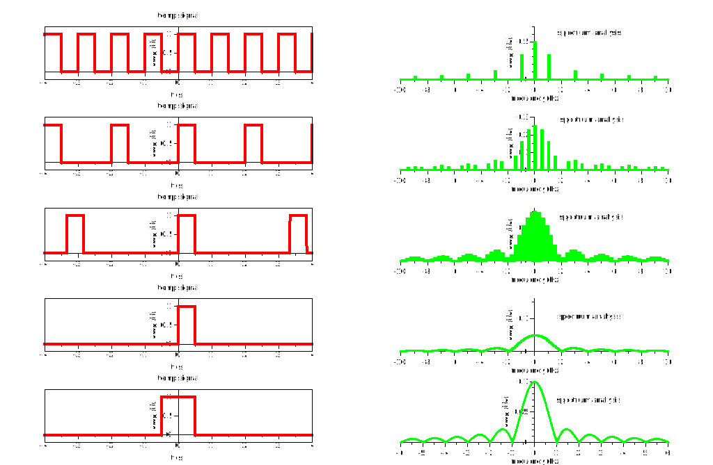
sftf.svg

y(t)=∑n=−∞+∞cnejnωt y(t)=\sum_{n=-\infty}^{+\infty}\color{red}{c_n} e^{jn\omega t}
y(t)=1T∑n=−∞+∞[∫−T2T2y(θ)e−j2πnθTdθ]ej2πntT y(t)=\frac{1}{T}\sum_{n=-\infty}^{+\infty}\color{red}{[\int_{-\frac{T}{2}}^{\frac{T}{2}}y(\theta)e^{-j\frac{2\pi n \theta}{T}} d\theta]}e^{j\frac{2\pi n t}{T}}
T→+∞=>nT→0=> T \rightarrow +\infty => \frac{n}{T} \rightarrow 0 => la somme discrète devient une somme continue

y(t)=∫−∞+∞[∫−∞+∞y(θ)e−j2πfθdθ]ej2πftdf y(t)=\int_{-\infty}^{+\infty}\color{red}{[\int_{-\infty}^{+\infty}y(\theta)e^{-j2\pi f \theta } d\theta]}e^{j2\pi ft} df
y(t)=∫−∞+∞Y(f)ej2πftdf y(t)=\int_{-\infty}^{+\infty}\color{red}{Y(f)}e^{j2\pi ft}df

Nous avions un spectre de raies pour un signal périodique ; ce spectre est continu pour un signal non périodique.


Définition de la transformée de Fourier

y(t)→FY(f) y(t) \overset{ \mathcal{F} }{\rightarrow}Y(f)

Y(f)=∫−∞+∞y(t)e−j2πftdt \boxed{ Y(f) = \int_{-\infty}^{+\infty}y(t)e^{-j2\pi f t } dt }

Y(f) constitue le spectre du signal Y.
C’est un nombre complexe .
Sur le schéma ci-dessus, seule l’amplitude est représentée ( il est possible si besoin de représenter également la phase ).


Exemple de transformées de fourier

δ(t)→F1 \delta(t)\overset{\mathcal{F}}{\rightarrow}1 : Le dirac excite toutes les fréquences

rect(t)→Fsinc(f)) rect(t)\overset{\mathcal{F}}{\rightarrow}sinc(f))

δ(t−t0)→F1 \delta(t-t_0)\overset{\mathcal{F}}{\rightarrow}1

IIITe→F1TeIIIfe III_{T_e}\overset{\mathcal{F}}{\rightarrow}\frac{1}{T_e}III_{f_e}

1→Fδ(f) 1\overset{\mathcal{F}}{\rightarrow}\delta(f)

ej2πf0t→Fδ(f−f0) e^{j2\pi f_0 t}\overset{\mathcal{F}}{\rightarrow}\delta(f-f_0)

sin⁡(2πf0t)→F12j[δ(f−f0)−δ(f+f0)] \sin(2\pi f_0 t)\overset{\mathcal{F}}{\rightarrow}\frac{1}{2j}[\delta(f-f_0)-\delta(f+f_0)]
cos⁡(2πf0t)→F12[δ(f−f0)+δ(f+f0)] \cos(2\pi f_0 t)\overset{\mathcal{F}}{\rightarrow}\frac{1}{2}[\delta(f-f_0)+\delta(f+f_0)]


Transformée de fourier d’une constante

Si je cherche directement la transformée de fourier d’une constante, je constate que le résultat est infini ( diverge ).

Approximation de la fonction constante :

g(t)=A.eϵ∣t∣ g(t)=A.e^{\epsilon |t|}
ϵ→0⇒g(t)→A \epsilon\rightarrow 0 \Rightarrow g(t)\rightarrow A
F[g(t)]=G(ω)=∫−∞0Aeϵte−jωtdt+∫0+∞Ae−ϵte−jωtdt \mathcal{F}[g(t)]=G(\omega)=\int_{-\infty}^{0}Ae^{\epsilon t}e^{-j\omega t}dt+\int_{0}^{+\infty}Ae^{-\epsilon t}e^{-j\omega t}dt
G(ω)=2ϵAϵ2+ω2 G(\omega)=\frac{2\epsilon A}{\epsilon^2+\omega^2}
ϵ→0⇒G(ω)=δ(ω) \epsilon \rightarrow 0 \Rightarrow G(\omega)=\delta(\omega)
∫−∞+∞2ϵAϵ2+ω2dω=2πA \int_{-\infty}^{+\infty}\frac{2\epsilon A}{\epsilon^2+\omega^2}d\omega = 2\pi A
F[A]=2πAδ(ω) \mathcal{F}[A]=2\pi A \delta(\omega)

On y arrive mais non sans mal …

Transformée de fourier de step

F[step(t)]=1jω+πδ(ω) \mathcal{F}[step(t)]=\frac{1}{j\omega}+\pi \delta(\omega)


Tranformée de fourier et convolution

y(t)=∫−∞∞x(τ)h(t−τ)dτ y(t)=\int_{-\infty}^{\infty}x(\tau)h(t-\tau)d\tau

Y(f)=∫−∞∞[∫−∞∞x(τ)h(t−τ)dτ]e−j2πftdt Y(f)=\int_{-\infty}^{\infty}\left[\int_{-\infty}^{\infty}x(\tau)h(t-\tau)d\tau\right]e^{-j2\pi f t} dt
Y(f)=∫−∞∞x(τ)[∫−∞∞h(t−τ)e−j2πftdt]dτ Y(f)=\int_{-\infty}^{\infty}x(\tau)\left[\int_{-\infty}^{\infty}h(t-\tau)e^{-j2\pi f t} dt\right]d\tau
ej2πfτe−j2πfτ=1 e^{j2\pi f \tau} e^{-j2\pi f \tau} = 1
Y(f)=∫−∞∞x(τ)e−j2πfτ[∫−∞∞h(t−τ)e−j2πftej2πfτdt]dτ Y(f)=\int_{-\infty}^{\infty}x(\tau)e^{-j2\pi f \tau} \left[\int_{-\infty}^{\infty}h(t-\tau)e^{-j2\pi f t} e^{ j2\pi f \tau} dt\right] d\tau
Y(f)=∫−∞∞x(τ)e−j2πfτ[∫−∞∞h(u)e−j2πfudu]dτ Y(f)=\int_{-\infty}^{\infty}x(\tau)e^{ -j2\pi f \tau} \left[\int_{-\infty}^{\infty}h(u)e^{-j2\pi f u} du\right] d\tau
Y(f)=[∫−∞∞x(τ)e−j2πfτdτ][∫−∞∞h(u)e−j2πfudu] Y(f)= \left[\int_{-\infty}^{\infty}x(\tau)e^{ -j2\pi f \tau} d\tau \right]\left[\int_{-\infty}^{\infty}h(u)e^{-j2\pi f u} du\right]

Y(f)=H(f).X(f) \boxed{ Y(f)=H(f).X(f) }

Produit de convolution en temporel–> Multiplication en TF

{F[step(t)]=1jω+πδ(ω)F[h(t)]=11+jωτ \left\{\begin{matrix} \mathcal{F}[step(t)]=\frac{1}{j\omega}+\pi \delta(\omega) \\ \mathcal{F}[h(t)]=\frac{1}{1+j\omega \tau} \end{matrix}\right.

F[y(t)]=F[h(t)⊗step(t)] \mathcal{F}[y(t)]=\mathcal{F}[h(t)\otimes step(t)]
Y(ω)=11+jωτ.(1jω+πδ(ω)) Y(\omega)=\frac{1}{1+j\omega \tau}.(\frac{1}{j\omega}+\pi \delta(\omega))
Y(ω)=1jω(1+jωτ)+πδ(ω)1+jωτ Y(\omega)=\frac{1}{j\omega(1+j\omega \tau)}+\frac{\pi \delta(\omega)}{1+j\omega \tau}
Y(ω)=1+jωτ−jωτjω(1+jωτ)+πδ(ω) Y(\omega)=\frac{1+j\omega \tau - j\omega \tau}{j\omega(1+j\omega \tau)}+\pi \delta(\omega)
Y(ω)=−τ1+jωτ+(1jω+πδ(ω)) Y(\omega)=-\frac{\tau}{1+j\omega\tau}+(\frac{1}{j\omega}+\pi\delta(\omega))
y(t)=F−1[Y(ω)]=step(t)−step(t)e−tτ y(t)= \mathcal{F}^{-1}[Y(\omega)]=step(t)-step(t)e^{-\frac{t}{\tau}}

y(t)=1−e−tτ pour t>0 \boxed{ y(t)= 1-e^{-\frac{t}{\tau}} \ pour \ t>0 }


Lien Fonction de Transfert <–> Transformée de Fourier de la réponse impulsionnelle

y(t)=h(t)⊗x(t) y(t)=h(t) \otimes x(t)

Pour x(t) fonction sinusoidale :

y(t)=∫−∞+∞h(τ).Aej2πf(t−τ)dτ y(t)=\int_{-\infty}^{+\infty} h(\tau).Ae^{j2\pi f(t-\tau)}d\tau
y(t)=Aej2πft∫−∞+∞h(τ).Aej2πf(−τ)dτ y(t)=Ae^{j2\pi ft}\color{red}{\int_{-\infty}^{+\infty} h(\tau).Ae^{j2\pi f(-\tau)}d\tau}
y(t)=Aej2πftH(f) y(t)=Ae^{j2\pi ft}\color{red}{H(f)}

Ainsi : La Transformée de Fourier de la réponse impulsionnelle d’un système correspond à sa fonction de Transfert


Transformée de Fourier d’un signal périodique –> Série de Fourier

Toute fonction périodique y(t) de période T peut s’écrire comme une somme infinie de cos et sin

y(t)=∑n=−∞+∞cnejnωt y(t)=\sum_{n=-\infty}^{+\infty}c_n e^{jn\omega t}
Y(f)=∫−∞+∞∑n=−∞+∞cnejnωte−j2πftdt Y(f) = \int_{-\infty}^{+\infty}\color{red}{\sum_{n=-\infty}^{+\infty}c_n e^{jn\omega t}}e^{-j2\pi f t } dt
Y(f)=∑n=−∞+∞cn∫−∞+∞ejnωte−j2πftdt Y(f) = \sum_{n=-\infty}^{+\infty} c_n \int_{-\infty}^{+\infty} e^{jn\omega t}e^{-j2\pi f t } dt
Y(f)=∑n=−∞+∞cnδ(f−nF) Y(f) = \sum_{n=-\infty}^{+\infty}c_n \delta(f-nF) –> Spectre de Raies (non continu) # série de fourier