Laplace : Placement des Poles

Nous avons observé précédemment un lien entre les pôles d’un système et la forme de la réponse temporelle.
Nous allons développer ce point dans cette partie.

Système du Premier Ordre

$H(s)=\frac{G}{1+\tau.s}$

considérons une entrée en échelon x(t)=step(t).

$Y(s)=H(s).X(s)$ avec $X(s)=\frac{1}{s}$

$Y(s)=\frac{G}{s(1+\tau.s)}$

$y(t)=G.(1-e^{-\frac{t}{\tau}})$

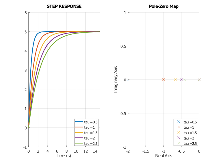
Influence de la constante de temps sur la réponse et évolution du pôle $-\frac{1}{\tau}$ :

Système du Second Ordre

$H(s)=\frac{G}{\frac{s^2}{\omega_n^2}+ \frac{2.\xi}{\omega_n}.s+1}$

$H(s)=\frac{G\omega_n^2}{s^2+ 2.\xi.\omega_n.s+\omega_n^2}$

$Y(s)=H(s).X(s)$ avec $X(s)=\frac{1}{s}$

Recherche des Pôles du système :

Résolution de :
$s^2+ 2.\xi.\omega_n.s+\omega_n^2 = 0$

RAPPEL:

Les solutions de l’équation $a.x^2+b.x+c = 0$ sont :

$\lambda_1=\frac{-b-\sqrt{\Delta}}{2a}$
$\lambda_2=\frac{-b+\sqrt{\Delta}}{2a}$

avec $\Delta = b^2 - 4ac$

Dans notre cas : $\Delta = \omega_n^2.(\xi^2-1)$

Cas $( \xi \gt 1 )$ –> 2 pôles Réels distincts

$\lambda_1=-\xi\omega_n+\omega_n\sqrt{\xi^2-1}$
$\lambda_2=-\xi\omega_n-\omega_n\sqrt{\xi^2-1}$
REMARQUE : stable si $\xi \geqslant 1$
$H(s)=\frac{G}{(1+T_1.s)(1+T_2.s)}$ , $T_1=-\frac{1}{\lambda_1}$ , $T_2=-\frac{1}{\lambda_2}$
$H(s)=\frac{K1}{1+T_1.s}-\frac{K2}{1+T_2.s}$ , $K_1=\frac{G.T_1}{T_1-T_2}, K_2=\frac{G.T_2}{T_1-T_2}$

$\boxed{ y(t)=K_1(1-e^{-\frac{t}{T_1}})-K_2(1-e^{-\frac{t}{T_2}}) }$

Cas $( \xi = 1 )$ –> 1 pôle réel double

$\lambda=-\xi\omega_n$

$\boxed{ y(t)=G\left[ 1-(1+\omega_n.t)e^{-\omega_n.t} \right] }$

Cas $( \xi \lt 1 )$ –> 2 pôles complexes conjugués

$\lambda_1=-\xi\omega_n-j.\omega_n\sqrt{1-\xi^2}$
$\lambda_2=-\xi\omega_n+j.\omega_n\sqrt{1-\xi^2}$
REMARQUE : stable si $0<\xi<1$

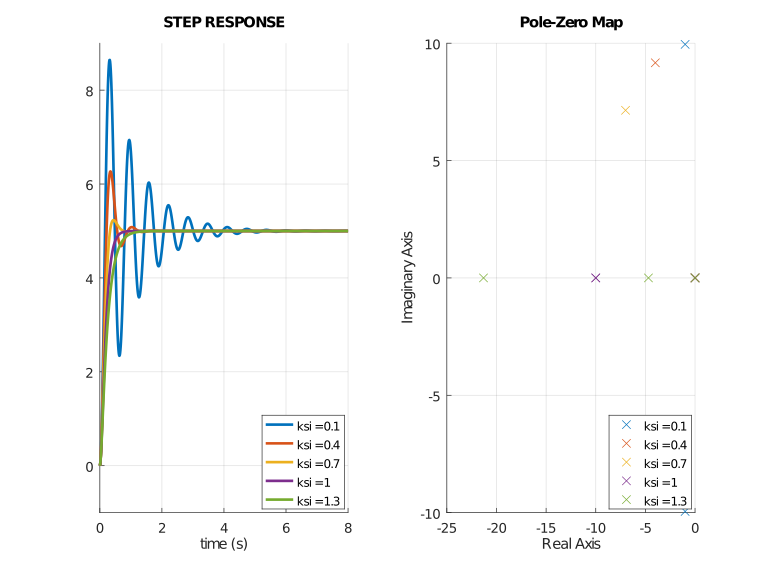
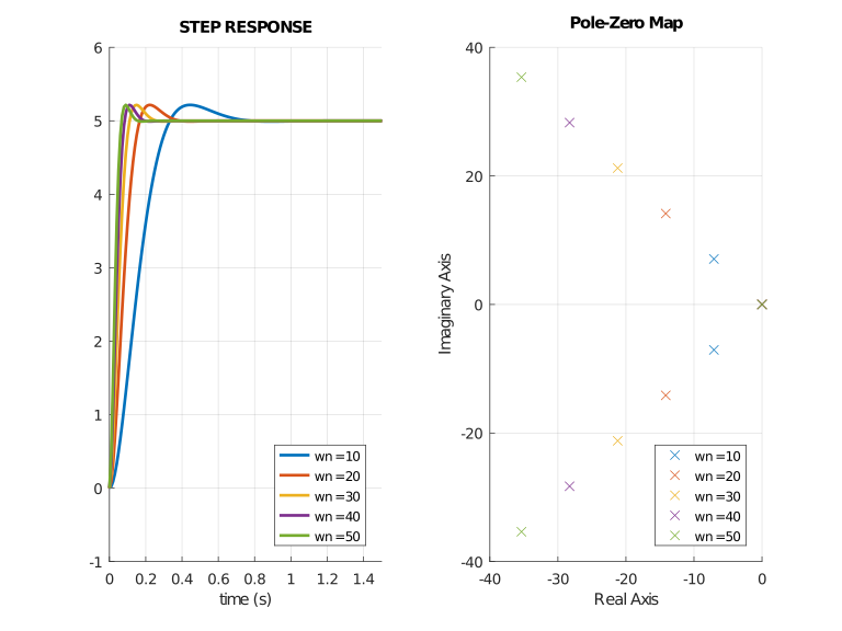
Réponse indicielle :

$\boxed{ y(t)=G\left ( 1-\frac{e^{-\xi\omega_nt}}{\sqrt{1-\xi^2 }}sin(\omega_p.t+\phi) \right ) }$

$\omega_p=\omega_n\sqrt{1-\xi^2}$
$\Phi=arctan{\frac{\sqrt{1-\xi^2}}{\xi}} = arccos(\xi)$

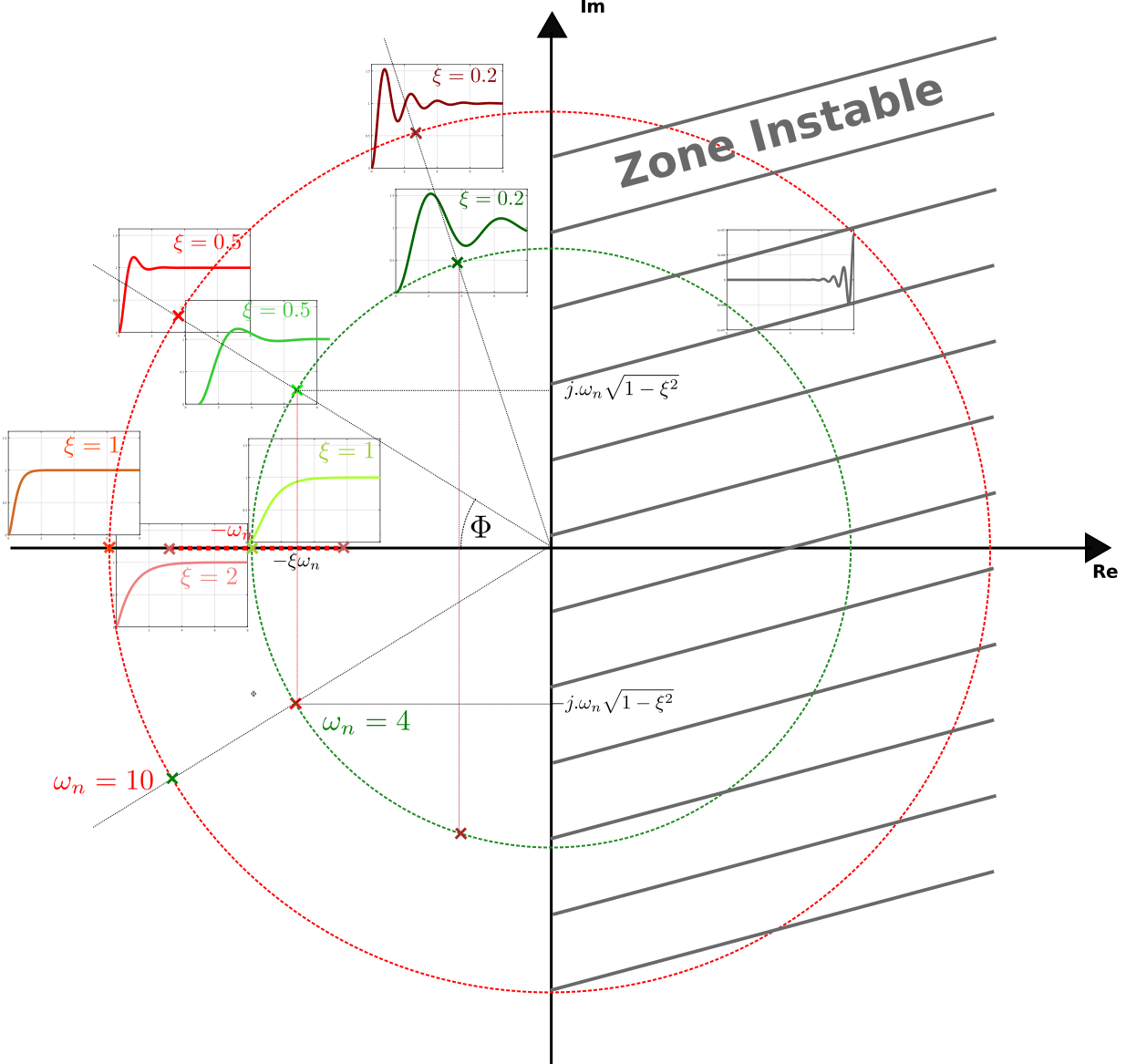
RESUME

Script Octave/Matlab pour générer les figures ci dessus

laplace_poles.m

laplace_poles.m

pkg load control
#====================================
G=5
tau=0.5
 
F = tf([G],[tau,1])
STEP= tf([1],[1,0])
t_end=15

t=0:0.01:t_end

figure(1)
%------------------------------------
subplot(1,2,1)

for i = 1:1:5
  F = tf([G],[tau,1])
  hold on
  p=step(F,t)   
  h=plot(t,p,'LineWidth',2,axis([0 t_end -1 6]))
  hold on
  LEG{i} = ['tau = ' num2str(tau)];
  hold on
  tau = tau + 0.5
end
     
legend(LEG,4);   
xlabel('time (s)')  
     
title('STEP RESPONSE')
grid
hold on
%------------------------------------
subplot(1,2,2)
tau=0.5

for i = 1:1:5
  F = tf([G],[tau,1])
  hold on
  pzmap(F*STEP, 'x')
  hold on
  LEG{i} = ['tau = ' num2str(tau)];
  hold on
  tau = tau + 0.5
end
legend(LEG,4);  

#print -deps premier_ordre.eps

#####################################
figure(2)

G=5
ksi=0.1 % Facteur d'amortissement
wn = 10 % pulsation naturelle non amortie

 
F = tf([G],[(1/wn)^2,((2*ksi)/wn),1])
STEP= tf([1],[1,0])
t_end=8

t=0:0.01:t_end

%------------------------------------
subplot(1,2,1)

for i = 1:1:5
  F = tf([G],[(1/wn)^2,((2*ksi)/wn),1])
  hold on
  p=step(F,t)   
  h=plot(t,p,'LineWidth',2,axis([0 t_end -1 9]))
  hold on
  LEG{i} = ['ksi = ' num2str(ksi)];
  hold on
  ksi = ksi+0.3
end
grid
legend(LEG,4);
title('STEP RESPONSE')
xlabel('time (s)')  

subplot(1,2,2)
ksi=0.1

for i = 1:1:5
  F = tf([G],[(1/wn)^2,((2*ksi)/wn),1])
  hold on
  pzmap(F*STEP, 'x')
  hold on
  LEG{i} = ['ksi = ' num2str(ksi)];
  hold on
  ksi = ksi+0.3
end
legend(LEG,4);

#####################################
figure(3)

G=5
ksi=sqrt(2)/2 % Facteur d'amortissement
wn = 10 % pulsation naturelle non amortie
 
F = tf([G],[(1/wn)^2,((2*ksi)/wn),1])
STEP= tf([1],[1,0])
t_end=8

t=0:0.01:t_end

%------------------------------------
subplot(1,2,1)
for i = 1:1:5
  F = tf([G],[(1/wn)^2,((2*ksi)/wn),1])
  hold on
  p=step(F,t)   
  h=plot(t,p,'LineWidth',2,axis([0 1.5 -1 6]))
  hold on
  LEG{i} = ['wn = ' num2str(wn)];
  hold on
  wn = wn+10
end
grid
legend(LEG,4);
title('STEP RESPONSE')
xlabel('time (s)')  
 
subplot(1,2,2)
ksi=sqrt(2)/2
wn = 10 % pulsation naturelle non amortie

for i = 1:1:5
  F = tf([G],[(1/wn)^2,((2*ksi)/wn),1])
  hold on
  pzmap(F*STEP, 'x')
  hold on
  LEG{i} = ['wn = ' num2str(wn)];
  hold on
  wn = wn+10
end
legend(LEG,4);
 
 print -dsvg second_ordre_wn.svg

#####################################

figure(4)

t_end=8

t=0:0.01:t_end

G=1
ksi=0.2% Facteur d'amortissement
wn = 10 % pulsation naturelle non amortie

F = tf([G],[(1/wn)^2,((2*ksi)/wn),1])
p=step(F,t)   
h=plot(t,p,'LineWidth',2)
axis([0 t_end 0 1.6])
grid

Transformée de Laplace Echantillonnage